More and more of the AI work I see touches images as well as text: document understanding, visual question answering, and agents that reason over screens, charts and scans. I wanted working fluency with vision-language models (VLMs) before recommending or building on them in client work, so I ran a focused deep dive and tried to answer four questions in order:
- How do these models actually work? I answered this by building one.
- What can a pretrained VLM do for a real structured-extraction problem, run locally, at acceptable accuracy and cost?
- How well can a VLM answer open-ended questions about a document it’s handed directly?
- How well does that hold up when the system first has to find the right document in a corpus?
The short version: model choice is the clearest driver of accuracy, and bigger or cloud-hosted isn’t always better. Once retrieval enters the picture, the retriever, not the generator, is usually the binding constraint.
A quick map of the field
I started with ten papers that trace how VLMs evolved. The throughline is short:
- CLIP proved images and text could share an embedding space, using contrastive training on 400 million image-caption pairs. Its vision encoder sits under almost every VLM since.
- Flamingo bridged a frozen vision encoder to a frozen LLM with heavy new adapter layers.
- BLIP-2 shrank that connector to a small Q-Former, matching Flamingo with 54× fewer trainable parameters.
- LLaVA reduced it to a single linear layer, fine-tuned the LLM itself, and used GPT-4 to generate synthetic instruction data.
- The current generation (Qwen2.5-VL, Qwen3-VL, InternVL3.5) treats connecting vision and language as largely solved, and focuses on dynamic resolution, long context, grounding, reasoning and agentic use.
- Molmo argues that data quality is the real lever. DeepSeek-OCR and DeepSeek-VL2 explore efficiency from opposite ends: one compresses the input (rendering text as an image to use far fewer tokens), the other compresses the compute with a mixture-of-experts model.
One more piece matters for retrieval later: ColPali, and its Qwen2-VL-based variant ColQwen2, embed whole page images and match queries against them with late interaction over patch embeddings, with no OCR at all. That keeps the layout, tables and charts that OCR flattens away.
Part I: building a VLM from scratch
Reading papers builds vocabulary. Building a model builds intuition for why the field’s design choices matter. I built a small VLM in three stages, trained each on the Flickr8k captioning dataset, and evaluated all three on the same fixed set of ten held-out images, so any improvement could be traced to the architectural change alone.
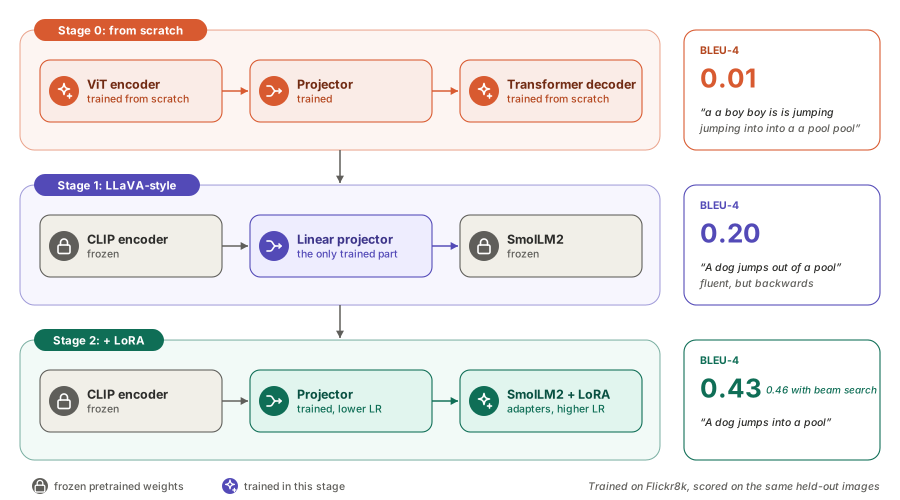
- Stage 0: from scratch. A Vision Transformer built directly in PyTorch (patch embedding, a CLS token, positional embeddings, pre-norm transformer blocks), a projection layer, and a transformer decoder, all trained from random initialisation.
- Stage 1: LLaVA-style, frozen backbones. A pretrained CLIP vision encoder and a small pretrained LLM (SmolLM2), both frozen, connected by one trainable linear layer. Image features become “visual tokens” prepended to the text through the LLM’s input embeddings, with no special cross-attention. Only the projector is trained.
- Stage 2: LoRA fine-tuning. Low-rank adapters on the LLM’s attention and MLP projections, trained together with the projector at different learning rates: lower for the already warm projector, higher for the new adapters. This is LLaVA’s second training stage in miniature.
I used corpus BLEU-4 on generated captions as the comparison metric, because it doesn’t depend on vocabulary or architecture. The from-scratch model and SmolLM2 use completely different tokenisers, so comparing their losses wouldn’t be meaningful.
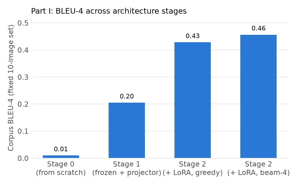
BLEU-4 went from 0.01 to 0.20 to 0.43, and switching Stage 2 to beam search pushed it to 0.46 with no retraining. The captions followed the same arc. For one image of a dog leaping into a pool after a ball:
- Stage 0: “a a boy boy is is jumping jumping into into a a pool pool”
- Stage 1: “A dog jumps out of a pool” (fluent, but backwards)
- Stage 2: “A dog jumps into a pool”
That’s the field’s central design decision, observed directly: frozen pretrained backbones joined by a lightweight connector, with a small trainable slice of the LLM, beat training everything from scratch by a wide margin. I stopped there on purpose. The goal was to show why the field converged on this recipe, not to optimise a captioning score.
Part II: local document field extraction
Next, a common enterprise task: extracting structured fields from scanned identity documents, using PAN and Aadhaar cards (Indian tax and national ID cards) from public datasets. The question was whether pretrained VLMs served entirely locally could be a credible first-tier option, before paying for larger cloud models.
I compared five models served locally with Ollama: Qwen2.5-VL 7B and 3B, Llama 3.2 Vision 11B, MiniCPM-V and LLaVA-Phi3 (the smallest model in the LLaVA family, as a link back to Part I). JSON-schema-constrained decoding guaranteed well-formed output without fragile prompt parsing.
Two things about real data shaped the evaluation:
- There was no ground truth at scale. The source annotations are bounding boxes, not field text. So I used two metrics: cross-model agreement (how often a model matches the majority answer across all five, on 100 images per document type) and manually transcribed ground truth on a labelled subsample.
- Dataset size isn’t diversity. The Aadhaar dataset had 1,852 files but only 217 distinct documents, some duplicated up to 17 times by augmentation. I deduplicated before sampling. A public dataset’s stated size can badly overstate its real variety, and it’s worth checking directly.
| Model | PAN agreement | PAN accuracy | Aadhaar agreement | Aadhaar accuracy | Latency (PAN / Aadhaar) |
|---|---|---|---|---|---|
| Qwen2.5-VL 7B | 98.5% | 86.7% | 95.9% | 66.7% | 17.4s / 4.4s |
| Qwen2.5-VL 3B | 91.0% | 46.7% | 87.1% | 46.7% | 13.3s / 2.8s |
| Llama 3.2 Vision 11B | 88.5% | 73.3% | 74.8% | 40.0% | 9.5s / 9.2s |
| MiniCPM-V | 76.2% | 40.0% | 71.8% | 13.3% | 5.1s / 3.8s |
| LLaVA-Phi3 | 7.5% | 0.0% | 30.3% | 0.0% | 7.5s / 10.0s |
What stood out:
- Qwen2.5-VL 7B won decisively on every metric for both document types. That’s consistent with its dynamic-resolution encoder and document-focused training.
- Cross-model agreement is a usable proxy for accuracy. The five models ranked identically on agreement and on hand-checked accuracy. That makes agreement a practical way to scale up evaluation when there are no labels.
- Aadhaar is harder than PAN for every model, with more fields and more layout variation.
- Speed and accuracy don’t trade off cleanly. The 3B Qwen model was about 25% faster on PAN but lost about 40 points of full-document accuracy.
The full sweep, about 1,000 model calls, took just under two hours. I ran it as a checkpointing script rather than notebook cells, so it could run unattended and resume after any interruption. That’s a small habit that pays off quickly.
Part III: question answering on a known document
Fixed fields are only part of the story. Real needs are open-ended questions over documents with no fixed schema. So I generalised to a single call: one image and one question in, one answer out. I tested it across six document types:
- PAN and Aadhaar cards, with each question anchored on another field of the same card (for example, “What is the full name of the person whose PAN number is X?”)
- Rental agreements: 43 real agreements rendered to page images, with questions written by hand after reading each one
- ChartQA: reading values and comparisons from bar and line charts
- SPIQA: questions about figures and tables in computer science papers
- MMLongBench-Doc: long, multi-page PDFs, about 20% of whose questions are deliberately unanswerable, to test whether a model declines instead of inventing an answer
I ran the same five local models plus two cloud models through OpenRouter: Gemini 3.1 Pro and Qwen2.5-VL 72B, the latter to see whether the local Qwen’s strength holds at ten times the size. Cloud runs used a smaller sample of 15 questions per dataset to control cost.
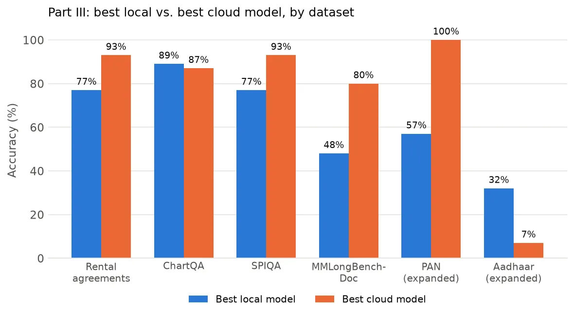
- No single model wins everywhere. Qwen2.5-VL 7B won ChartQA outright (89%, beating both cloud models), but MiniCPM-V beat it on SPIQA (77% vs 63%) and Aadhaar, and Llama 3.2 Vision edged it on MMLongBench-Doc. Part II’s clear winner didn’t automatically generalise. The right model depends on the document type.
- Cloud isn’t a safe default. Cloud models won clearly on rental agreements, SPIQA and long documents, but lost on ChartQA and, dramatically, on Aadhaar.
- Given the right document, most models read most documents well. PAN, rental agreements, ChartQA and SPIQA all had at least one model above 80%.
- Aadhaar is the exception. Even Gemini 3.1 Pro (7%) and Qwen2.5-VL 72B (0%) failed when handed the right card directly. I haven’t yet isolated why, whether it’s layout density, print quality or the template itself, but it’s a reading problem that more ground truth alone won’t fix.
Two practical warnings came out of this part. First, serving-stack bugs can masquerade as model weakness. In my local setup, one model crashed on many multi-image calls, and two others sometimes returned a “successful” response with an empty answer. That’s invisible to simple error monitoring, because no error is logged. Second, latency has a long tail. One configuration averaged 353 seconds on ChartQA but had a median of 15. For a deployment conversation, the median is the honest number.
Part IV: retrieval-augmented visual QA
A real system isn’t handed the right document. It has to find it from the question alone. So I added a retrieval step in front of generation: a visual RAG system in the ColPali sense.
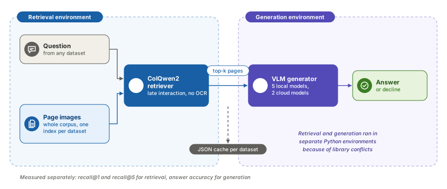
- Retrieval: ColQwen2 indexes every page image in a dataset’s corpus, and each question searches the whole corpus, never just the document it came from. That’s both realistic and what makes recall@k meaningful.
- Generation: the same seven models, answering from whatever pages retrieval actually returned.
- Engineering: ColPali’s library pins conflicted with the main project’s, so retrieval and generation ran in separate Python environments, communicating only through a small JSON cache file per dataset.
I deliberately chose visual retrieval over the more conventional route of OCR followed by text RAG. OCR throws away exactly the layout information that tables, charts and ID cards depend on. I didn’t build or benchmark the text-RAG alternative.
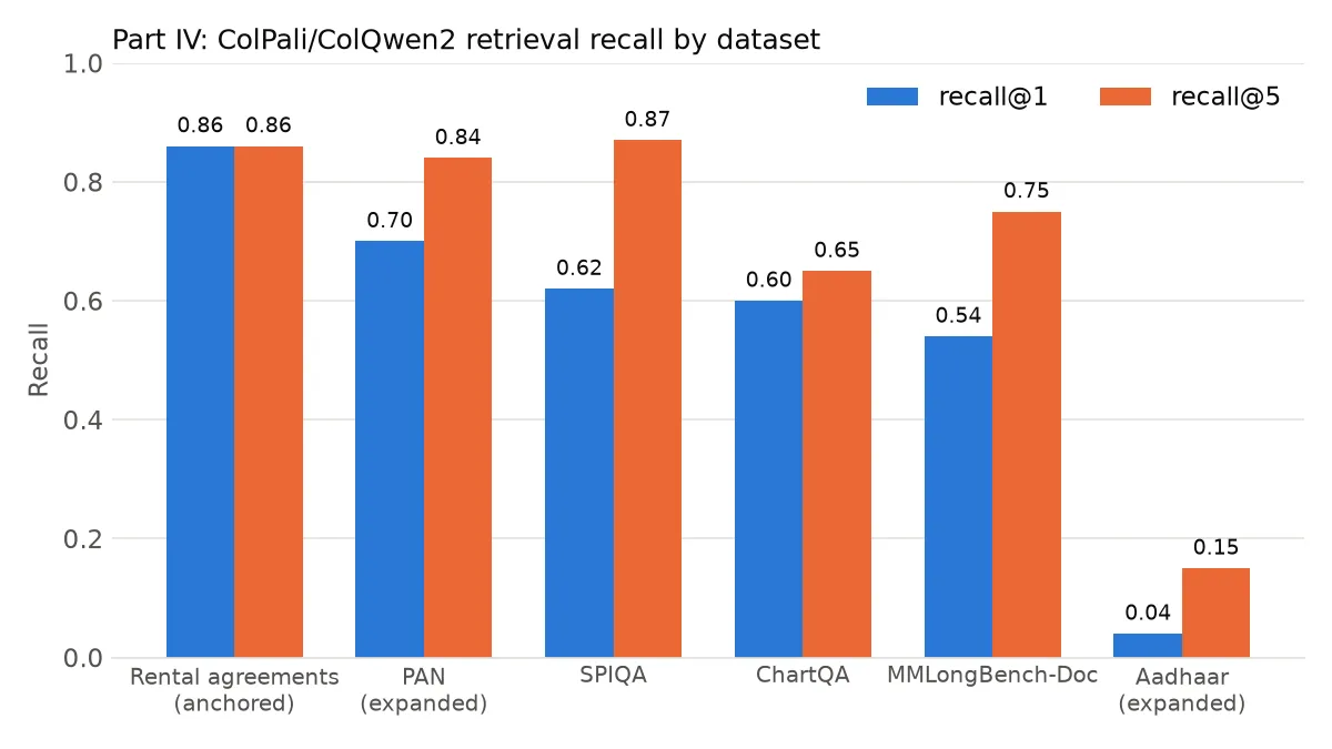
| Dataset | recall@1 | recall@5 |
|---|---|---|
| Rental agreements (anchored questions) | 0.86 | 0.86 |
| PAN | 0.70 | 0.84 |
| SPIQA | 0.62 | 0.87 |
| ChartQA | 0.60 | 0.65 |
| MMLongBench-Doc | 0.54 | 0.75 |
| Aadhaar | 0.04 | 0.15 |
Comparing accuracy with the right document handed over (Part III’s “oracle” setting) against accuracy on the retrieved pages, for the same questions, shows where the losses come from:
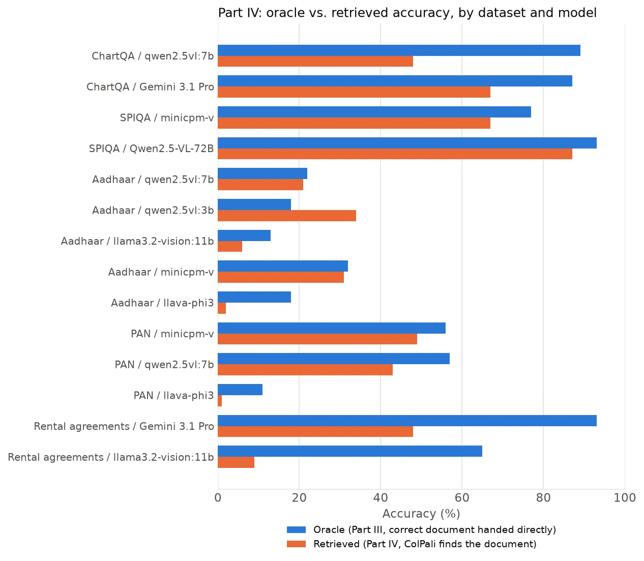
- Retrieval is usually the binding constraint. On ChartQA, Qwen2.5-VL 7B dropped from 89% with the right chart to 48% with retrieved ones. Gemini 3.1 Pro dropped from 87% to 67%. Same model, same question; only the source of the image changed. When a visual RAG system gives a disappointing answer, check whether retrieval found the right page before blaming the generator.
- PAN pays a moderate retrieval tax (for example, 56% to 49% for MiniCPM-V), consistent with its recall@1 of 0.70.
- Anchored questions are easier to retrieve. Rental-agreement questions anchored to a distinguishing detail, such as an execution date or a named party, reached recall@1 of 0.86. With the original, generic questions, retrieved accuracy collapsed: Gemini 3.1 Pro fell from 93% to 48%. That’s an actionable rule for writing retrieval evaluation sets.
- Aadhaar has two compounding weaknesses. Retrieval is near chance (two cards came out top for about two-thirds of unrelated questions), and generation is weak even with the right card. Fixing retrieval alone wouldn’t rescue it.
- ColQwen2 is workable but has headroom. Outside Aadhaar, recall@1 ranged from 0.54 to 0.70: the top guess is right roughly two times in three at best.
I also wrapped both phases in Gradio tools, one for asking a question about a single image and one for the full retrieve-then-generate pipeline, showing the retrieved pages and their scores. Seeing the retrieved pages next to the answer made the “it found the wrong page” failure mode obvious in a way a metric alone doesn’t.
Lessons learned
- Build it once to understand it. A small from-scratch VLM made the frozen-backbone, lightweight-connector recipe concrete in a way no paper did.
- Pick the model per task, not by size or vendor. The best model changed with the document type, and a well-chosen local 7B model beat cloud models on some tasks.
- When there are no labels, agreement can stand in, if you validate it. Cross-model agreement ranked models exactly as hand-checked accuracy did.
- Check your data, not just its description. One dataset’s 1,852 files were 217 documents.
- Separate retrieval from generation when you evaluate. Measuring the oracle and retrieved settings on the same questions is what shows which half needs the investment.
- In visual RAG, invest in the retriever first. It was more often the bottleneck than the generator, and it has the most obvious room to improve.
- Watch the serving stack. Silent empty answers and crashes can distort a model comparison. Report medians, not just averages.
What’s next
The obvious next step is to improve retrieval rather than just diagnose it:
- Re-ranking ColQwen2’s top results with a cross-encoder or the VLM itself
- Hybrid retrieval that fuses OCR text search with visual embeddings
- Higher-resolution or multi-crop indexing for documents with small print
- Fine-tuning ColQwen2 on these specific document types
I’d also like to extend the cloud comparison to the Part II extraction task, which so far has only been run locally because of cost.
The takeaway
VLMs are capable readers when they’re given the right page and the right model is chosen for the task. The harder engineering problem in a real system is finding that page. If you’re putting a VLM in front of a document corpus, measure your retriever as carefully as your generator, and expect to spend more of your effort there.
If you’re working with vision-language models, I’d love to compare notes. Find me on LinkedIn.